Hello @mdal,
What you are looking to do is definitely feasible within R. Below is an example of how I would tackle the problem. However, there are two options to generalize: you could write a function that takes the years you want to include in the 5-year average calculation and then another to take the years you want to include as counts. Alternatively, you could try using the slider package to calculate 5-year rolling averages for each year.
# loading packages
library(tidyverse)
library(gt)
# creating linelist data
linelist_data <- tibble(
year = sample(
x = 2015:2021,
size = 500,
replace = TRUE
),
disease = sample(
x = c("Disease A", "Disease B"),
size = 500,
replace = TRUE
),
sex = sample(
x = c("Female", "Male"),
size = 500,
replace = TRUE
),
age_group = sample(
x = c("0-14", "15-29", "30-39", "40-49", ">=50"),
size = 500,
replace = TRUE
),
n = rpois(n = 500, lambda = 65)
) |>
mutate(
disease = factor(x = disease, levels = c("Disease A", "Disease B")),
sex = factor(x = sex, levels = c("Female", "Male")),
age_group = factor(age_group, levels = c("0-14", "15-29", "30-39", "40-49", ">=50"))
)
# aggregating linelist data
aggregated_data <- linelist_data |>
count(disease,
year,
sex,
age_group) |>
complete(disease,
year = 2015:2021,
sex,
age_group,
fill = list(n = 0))
# creating average data for 2015 to 2019
averages <- aggregated_data |>
filter(between(year, 2015, 2019)) |>
group_by(disease,
sex,
age_group) |>
summarise(average = mean(n),
.groups = "drop")
# creating counts data for 2020 and 2021 in a wide format
counts <- aggregated_data |>
filter(between(year, 2020, 2021)) |>
pivot_wider(
id_cols = c(disease, sex, age_group),
names_prefix = "count_",
names_from = year,
values_from = n
)
# joining the counts and average data, you can adjust how trend is defined
joined_data <- counts |>
left_join(averages,
by = c("disease", "sex", "age_group")) |>
mutate(
trend_2020 = sign(count_2020 - average),
trend_2021 = sign(count_2021 - average)
) |>
relocate(disease,
sex,
age_group,
average,
count_2020,
trend_2020,
count_2021,
trend_2021)
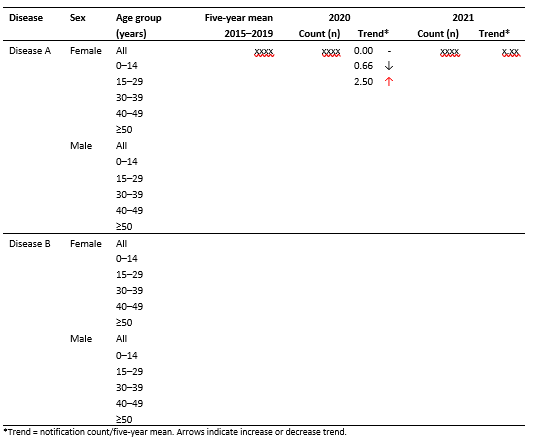
# using gt to create a nice table - you could look into creating group rows
joined_data |>
gt() |>
cols_label(
disease = "Disease",
sex = "Sex",
age_group = "Age Group",
average = "5 year mean",
count_2020 = "Count",
trend_2020 = "Trend",
count_2021 = "Count",
trend_2021 = "Trend"
) |>
tab_spanner(label = "2020",
columns = c("count_2020", "trend_2020")) |>
tab_spanner(label = "2021",
columns = c("count_2021", "trend_2021"))
Created on 2022-05-19 by the reprex package (v2.0.1)
Session info
sessioninfo::session_info()
#> ─ Session info ───────────────────────────────────────────────────────────────
#>  setting  value
#>  version  R version 4.1.3 (2022-03-10)
#>  os       macOS Big Sur/Monterey 10.16
#>  system   x86_64, darwin17.0
#>  ui       X11
#>  language (EN)
#>  collate  en_CA.UTF-8
#>  ctype    en_CA.UTF-8
#>  tz       America/Toronto
#>  date     2022-05-19
#>  pandoc   2.17.1.1 @ /Applications/RStudio.app/Contents/MacOS/quarto/bin/ (via rmarkdown)
#>
#> ─ Packages ───────────────────────────────────────────────────────────────────
#>  package     * version date (UTC) lib source
#>  assertthat    0.2.1   2019-03-21 [1] CRAN (R 4.1.0)
#>  backports     1.4.1   2021-12-13 [1] CRAN (R 4.1.0)
#>  broom         0.8.0   2022-04-13 [1] CRAN (R 4.1.3)
#>  cellranger    1.1.0   2016-07-27 [1] CRAN (R 4.1.0)
#>  checkmate     2.1.0   2022-04-21 [1] CRAN (R 4.1.3)
#>  cli           3.3.0   2022-04-25 [1] CRAN (R 4.1.3)
#>  colorspace    2.0-3   2022-02-21 [1] RSPM (R 4.1.2)
#>  crayon        1.5.1   2022-03-26 [1] CRAN (R 4.1.3)
#>  DBI           1.1.2   2021-12-20 [1] CRAN (R 4.1.1)
#>  dbplyr        2.1.1   2021-04-06 [1] CRAN (R 4.1.0)
#>  digest        0.6.29  2021-12-01 [1] CRAN (R 4.1.1)
#>  dplyr       * 1.0.9   2022-04-28 [1] CRAN (R 4.1.3)
#>  ellipsis      0.3.2   2021-04-29 [1] CRAN (R 4.1.0)
#>  evaluate      0.15    2022-02-18 [1] RSPM (R 4.1.2)
#>  fansi         1.0.3   2022-03-24 [1] CRAN (R 4.1.3)
#>  fastmap       1.1.0   2021-01-25 [1] CRAN (R 4.1.0)
#>  forcats     * 0.5.1   2021-01-27 [1] CRAN (R 4.1.0)
#>  fs            1.5.2   2021-12-08 [1] CRAN (R 4.1.1)
#>  generics      0.1.2   2022-01-31 [1] RSPM (R 4.1.2)
#>  ggplot2     * 3.3.6   2022-05-03 [1] CRAN (R 4.1.3)
#>  glue          1.6.2   2022-02-24 [1] RSPM (R 4.1.2)
#>  gt          * 0.5.0   2022-04-21 [1] CRAN (R 4.1.3)
#>  gtable        0.3.0   2019-03-25 [1] CRAN (R 4.1.0)
#>  haven         2.5.0   2022-04-15 [1] CRAN (R 4.1.3)
#>  highr         0.9     2021-04-16 [1] CRAN (R 4.1.0)
#>  hms           1.1.1   2021-09-26 [1] CRAN (R 4.1.1)
#>  htmltools     0.5.2   2021-08-25 [1] CRAN (R 4.1.0)
#>  httr          1.4.3   2022-05-04 [1] CRAN (R 4.1.2)
#>  jsonlite      1.8.0   2022-02-22 [1] RSPM (R 4.1.2)
#>  knitr         1.39    2022-04-26 [1] CRAN (R 4.1.3)
#>  lifecycle     1.0.1   2021-09-24 [1] CRAN (R 4.1.1)
#>  lubridate     1.8.0   2021-10-07 [1] CRAN (R 4.1.1)
#>  magrittr      2.0.3   2022-03-30 [1] CRAN (R 4.1.3)
#>  modelr        0.1.8   2020-05-19 [1] CRAN (R 4.1.0)
#>  munsell       0.5.0   2018-06-12 [1] CRAN (R 4.1.0)
#>  pillar        1.7.0   2022-02-01 [1] RSPM (R 4.1.2)
#>  pkgconfig     2.0.3   2019-09-22 [1] CRAN (R 4.1.0)
#>  purrr       * 0.3.4   2020-04-17 [1] CRAN (R 4.1.0)
#>  R.cache       0.15.0  2021-04-30 [1] CRAN (R 4.1.0)
#>  R.methodsS3   1.8.1   2020-08-26 [1] CRAN (R 4.1.0)
#>  R.oo          1.24.0  2020-08-26 [1] CRAN (R 4.1.0)
#>  R.utils       2.11.0  2021-09-26 [1] CRAN (R 4.1.1)
#>  R6            2.5.1   2021-08-19 [1] CRAN (R 4.1.0)
#>  readr       * 2.1.2   2022-01-30 [1] RSPM (R 4.1.2)
#>  readxl        1.4.0   2022-03-28 [1] CRAN (R 4.1.3)
#>  reprex        2.0.1   2021-08-05 [1] CRAN (R 4.1.0)
#>  rlang         1.0.2   2022-03-04 [1] CRAN (R 4.1.2)
#>  rmarkdown     2.14    2022-04-25 [1] CRAN (R 4.1.3)
#>  rstudioapi    0.13    2020-11-12 [1] CRAN (R 4.1.0)
#>  rvest         1.0.2   2021-10-16 [1] CRAN (R 4.1.1)
#>  sass          0.4.1   2022-03-23 [1] CRAN (R 4.1.2)
#>  scales        1.2.0   2022-04-13 [1] CRAN (R 4.1.3)
#>  sessioninfo   1.2.2   2021-12-06 [1] CRAN (R 4.1.1)
#>  stringi       1.7.6   2021-11-29 [1] CRAN (R 4.1.1)
#>  stringr     * 1.4.0   2019-02-10 [1] CRAN (R 4.1.0)
#>  styler        1.7.0   2022-03-13 [1] CRAN (R 4.1.2)
#>  tibble      * 3.1.7   2022-05-03 [1] CRAN (R 4.1.3)
#>  tidyr       * 1.2.0   2022-02-01 [1] RSPM (R 4.1.2)
#>  tidyselect    1.1.2   2022-02-21 [1] RSPM (R 4.1.2)
#>  tidyverse   * 1.3.1   2021-04-15 [1] CRAN (R 4.1.0)
#>  tzdb          0.3.0   2022-03-28 [1] CRAN (R 4.1.3)
#>  utf8          1.2.2   2021-07-24 [1] CRAN (R 4.1.0)
#>  vctrs         0.4.1   2022-04-13 [1] CRAN (R 4.1.3)
#>  withr         2.5.0   2022-03-03 [1] RSPM (R 4.1.2)
#>  xfun          0.31    2022-05-10 [1] CRAN (R 4.1.3)
#>  xml2          1.3.3   2021-11-30 [1] CRAN (R 4.1.1)
#>  yaml          2.3.5   2022-02-21 [1] RSPM (R 4.1.2)
#>
#>  [1] /Users/timothychisamore/Library/R/x86_64/4.1/library
#>  [2] /Library/Frameworks/R.framework/Versions/4.1/Resources/library
#>
#> ──────────────────────────────────────────────────────────────────────────────
All the best,
Tim