Overview of steps
-
Do your research first
Search for an answer in Applied Epi’s free Epidemiologist R Handbook, the R for Data Science book, or by searching on Stack Overflow. Write in your post about your attempts to find answers elsewhere (with links). -
Summarize your problem so that readers can re-create it on their own computers
- Provide a complete “reproducible example” using the guidance below. You are much more likely to get a useful answer!
- Do not include sensitive or personal data in your post
- If you just want to type or paste a small amount of code, you can do this within three backticks
(note that a backtick ` is different from a single quote mark ’ and is usually found on the ~ key)
```
linelist <- linelist_raw %>%
   filter(gender == "Male") %>%
   select(case_id, age, gender, outcome)
```
-
Add “tags” to your question so that others can easily find it (e.g. Data cleaning, R Markdown, Shiny, etc.)
-
Thank those who volunteered their time to provide an answer.
How to create a “reproducible example”:
Make it easy for people to help you. Give readers a way to re-create your problem on their own computer with a “minimal, reproducible example” of your problem:
- Be minimal - include only the data and code required to reproduce your problem
- Be reproducible - include all data and package commands, e.g.
library()orp_load()
The two steps described below are:
1. Decide which data to use
Use part of your dataset that is in R
The {datapasta} converts a small portion of your dataset into code, which you can paste into your reproducible example so that readers can re-create this portion of your dataset within their own computer.
Decide which small part of your data to share. ![]() Think seriously about whether you are allowed to share it. Ensure there is no patient, identifiable, or otherwise sensitive information.
Think seriously about whether you are allowed to share it. Ensure there is no patient, identifiable, or otherwise sensitive information.
Install and load the {datapasta} package
install.packages("datapasta")
library(datapasta)
Save a small part of your data as an object in your Environment, with a name (e.g. “demo_data”). Choose only enough data to demonstrate your problem.
demo_data <- my_linelist %>%
   head(10) %>%                         # keep only first 10 rows
   select(case_id, gender, onset_date)  # keep only certain columns
Run the function dpasta() on your object, like this:
dpasta(demo_data)
Now, in your R script there will appear a command to re-create the data. You can paste this code into your “reproducible example” (see below) so that others can re-create and solve your problem.
data.frame(
  stringsAsFactors = FALSE,
           case_id = c("694928","86340d","92d002",
                       "544bd1","6056ba","eb5aeb","e64e04","5a65bb","2ae019",
                       "7ca4c0"),
            gender = c("m", "f", "f", "f", "f", "f", "f", "m", "m", "m"),
        onset_date = c("11/9/2014","10/30/2014",
                       "8/16/2014","8/29/2014","10/20/2014","10/28/2014",
                       "10/6/2014","9/21/2014","5/6/2014","9/29/2014")
)
Or, click here to use data in Excel
Alternatively, follow the instructions above to install and load {datapasta}, then go to your raw data (e.g. in an Excel file), copy only the data you want to include, and run the tribble_paste() function in your R script (with empty parentheses). This command will produce a command in your script that produces the data that was on your clipboard, in R.
tribble_paste()
For example, if this Excel data selection copied to your clipboard:
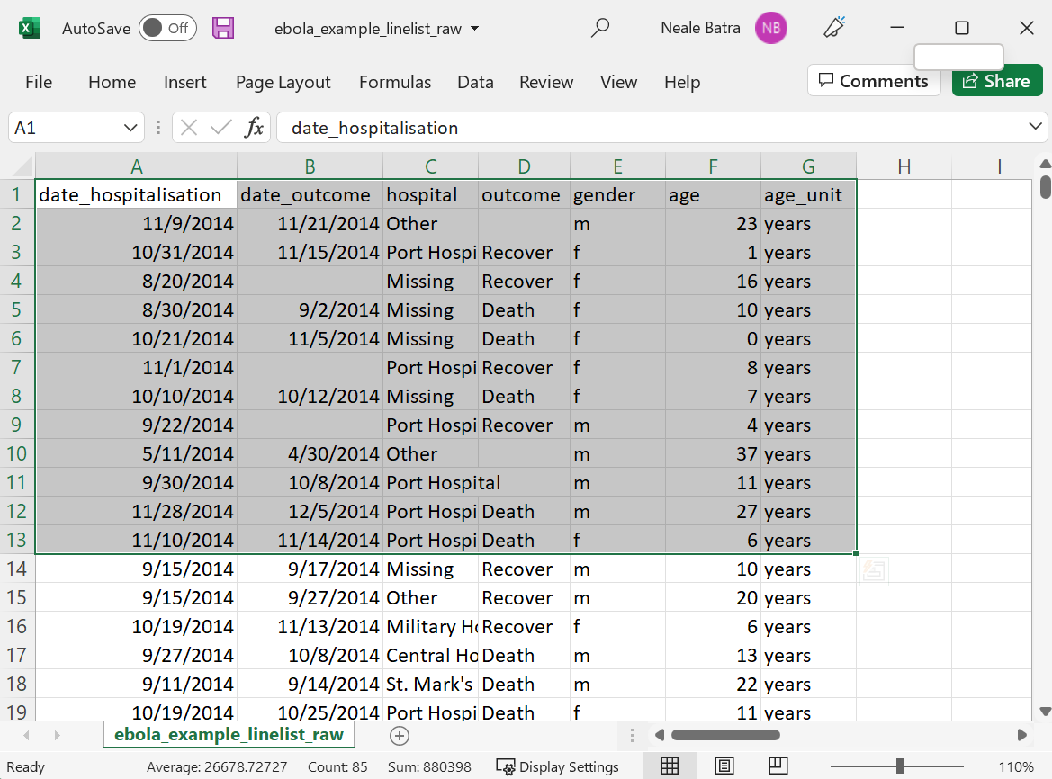
This code will be produced when the command tribble_paste() is run in your R script:
tibble::tribble(
  ~date_hospitalisation, ~date_outcome,       ~hospital,  ~outcome, ~gender, ~age, ~age_unit,
            "11/9/2014",  "11/21/2014",         "Other",        NA,     "m",  23L,   "years",
           "10/31/2014",  "11/15/2014", "Port Hospital", "Recover",     "f",   1L,   "years",
            "8/20/2014",            NA,       "Missing", "Recover",     "f",  16L,   "years",
            "8/30/2014",    "9/2/2014",       "Missing",   "Death",     "f",  10L,   "years",
           "10/21/2014",   "11/5/2014",       "Missing",   "Death",     "f",   0L,   "years",
            "11/1/2014",            NA, "Port Hospital", "Recover",     "f",   8L,   "years",
           "10/10/2014",  "10/12/2014",       "Missing",   "Death",     "f",   7L,   "years",
            "9/22/2014",            NA, "Port Hospital", "Recover",     "m",   4L,   "years",
            "5/11/2014",   "4/30/2014",         "Other",        NA,     "m",  37L,   "years",
            "9/30/2014",   "10/8/2014", "Port Hospital",        NA,     "m",  11L,   "years",
           "11/28/2014",   "12/5/2014", "Port Hospital",   "Death",     "m",  27L,   "years",
           "11/10/2014",  "11/14/2014", "Port Hospital",   "Death",     "f",   6L,   "years"
  )
You can add an assignment operator at the top of the code, e.g. mydata <- tibble::tribble( to name your dataset and reference it in later commands.
Or, click here to use a public dataset
Another simple and safe option is to use one of the publicly-available datasets to pose your question:
- Run
data()to see R’s built-in datasets, OR - Install the {outbreaks} R package and use one of its many datasets - for example by running
install.packages("outbreaks")and thenoutbreaks::fluH7N9_china_2013 - Use one of Applied Epi’s public health datasets.
2. Now, make an example with the {reprex} package
The {reprex} package (part of the tidyverse) can assist you with making a reproducible example:
# install and then load {tidyverse} (which includes the {reprex} package)
install.packages("tidyverse")   # install if necessary
library(tidyverse)              # load for use
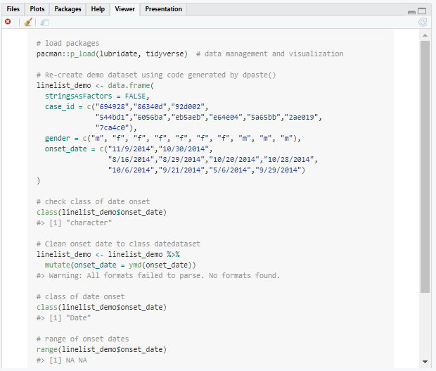
Write a simple, minimal R script that recreates your problem. Start by loading packages, and create a small dataset for the example (see the above techniques using the {datapasta} package).
In the example below, we load packages with pacman::p_load(), use code generated by dpaste() to re-create a small part of our case linelist, then use mutate() and ymd() to try to convert the column onset_date from character to date class. However, we are confused why all the dates have been converted to NA!
# load packages
pacman::p_load(lubridate, tidyverse)  # data management and visualization

# Re-create demo dataset using code generated by dpaste()
linelist_demo <- data.frame(
  stringsAsFactors = FALSE,
  case_id = c("694928","86340d","92d002",
              "544bd1","6056ba","eb5aeb","e64e04","5a65bb","2ae019",
              "7ca4c0"),
  gender = c("m", "f", "f", "f", "f", "f", "f", "m", "m", "m"),
  onset_date = c("11/9/2014","10/30/2014",
                 "8/16/2014","8/29/2014","10/20/2014","10/28/2014",
                 "10/6/2014","9/21/2014","5/6/2014","9/29/2014")
)

# check class of date onset
class(linelist_demo$onset_date)

# Clean onset date to class datedataset
linelist_demo <- linelist_demo %>%
  mutate(onset_date = ymd(onset_date))

# class of date onset
class(linelist_demo$onset_date)

# range of onset dates (why are all the dates NA?!)
range(linelist_demo$onset_date)
Now, copy all the relevant code from your script to your clipboard, and run the following command:
reprex(session_info = TRUE)
You will see an HTML output appear in the RStudio Viewer pane. It will contain all your code and any warnings, errors, or plot outputs. This output is also copied to your clipboard, so you can paste it directly into an Applied Epi Community post or Github post.
Someone can copy your example and run it in their own computer. They can explain that we needed to use the {lubridate} function mdy() to convert onset_date column to date class, not ymd(), because the raw dates are written in the format month-day-year.
If you paste the “reprex” into an Applied Epi Community post, it will look like below. Other people can now re-create your problem, and tell you how to fix it!
# load packages
pacman::p_load(lubridate, tidyverse)  # data management and visualization

# Re-create demo dataset using code generated by dpaste()
linelist_demo <- data.frame(
  stringsAsFactors = FALSE,
  case_id = c("694928","86340d","92d002",
              "544bd1","6056ba","eb5aeb","e64e04","5a65bb","2ae019",
              "7ca4c0"),
  gender = c("m", "f", "f", "f", "f", "f", "f", "m", "m", "m"),
  onset_date = c("11/9/2014","10/30/2014",
                 "8/16/2014","8/29/2014","10/20/2014","10/28/2014",
                 "10/6/2014","9/21/2014","5/6/2014","9/29/2014")
)

# check class of date onset
class(linelist_demo$onset_date)
#> [1] "character"

# Clean onset date to class datedataset
linelist_demo <- linelist_demo %>%
  mutate(onset_date = ymd(onset_date))
#> Warning: All formats failed to parse. No formats found.

# class of date onset
class(linelist_demo$onset_date)
#> [1] "Date"

# range of onset dates
range(linelist_demo$onset_date)
#> [1] NA NA
Created on 2022-09-16 by the reprex package (v2.0.1)
Session info
sessioninfo::session_info()
#> ─ Session info ───────────────────────────────────────────────────────────────
#>  setting  value
#>  version  R version 4.2.1 (2022-06-23 ucrt)
#>  os       Windows 10 x64 (build 22000)
#>  system   x86_64, mingw32
#>  ui       RTerm
#>  language (EN)
#>  collate  English_United States.utf8
#>  ctype    English_United States.utf8
#>  tz       Europe/Berlin
#>  date     2022-09-16
#>  pandoc   2.18 @ C:/Program Files/RStudio/bin/quarto/bin/tools/ (via rmarkdown)
#>
#> ─ Packages ───────────────────────────────────────────────────────────────────
#>  package       * version date (UTC) lib source
#>  assertthat      0.2.1   2019-03-21 [1] CRAN (R 4.2.1)
#>  backports       1.4.1   2021-12-13 [1] CRAN (R 4.2.0)
#>  broom           1.0.0   2022-07-01 [1] CRAN (R 4.2.1)
#>  cellranger      1.1.0   2016-07-27 [1] CRAN (R 4.2.1)
#>  cli             3.3.0   2022-04-25 [1] CRAN (R 4.2.1)
#>  colorspace      2.0-3   2022-02-21 [1] CRAN (R 4.2.1)
#>  crayon          1.5.1   2022-03-26 [1] CRAN (R 4.2.1)
#>  curl            4.3.2   2021-06-23 [1] CRAN (R 4.2.1)
#>  DBI             1.1.3   2022-06-18 [1] CRAN (R 4.2.1)
#>  dbplyr          2.2.1   2022-06-27 [1] CRAN (R 4.2.1)
#>  digest          0.6.29  2021-12-01 [1] CRAN (R 4.2.1)
#>  dplyr         * 1.0.9   2022-04-28 [1] CRAN (R 4.2.1)
#>  ellipsis        0.3.2   2021-04-29 [1] CRAN (R 4.2.1)
#>  evaluate        0.16    2022-08-09 [1] CRAN (R 4.2.1)
#>  fansi           1.0.3   2022-03-24 [1] CRAN (R 4.2.1)
#>  fastmap         1.1.0   2021-01-25 [1] CRAN (R 4.2.1)
#>  forcats       * 0.5.2   2022-08-19 [1] CRAN (R 4.2.1)
#>  fs              1.5.2   2021-12-08 [1] CRAN (R 4.2.1)
#>  gargle          1.2.0   2021-07-02 [1] CRAN (R 4.2.1)
#>  generics        0.1.3   2022-07-05 [1] CRAN (R 4.2.1)
#>  ggplot2       * 3.3.6   2022-05-03 [1] CRAN (R 4.2.1)
#>  glue            1.6.2   2022-02-24 [1] CRAN (R 4.2.1)
#>  googledrive     2.0.0   2021-07-08 [1] CRAN (R 4.2.1)
#>  googlesheets4   1.0.0   2021-07-21 [1] CRAN (R 4.2.1)
#>  gtable          0.3.1   2022-09-01 [1] CRAN (R 4.2.1)
#>  haven           2.5.0   2022-04-15 [1] CRAN (R 4.2.1)
#>  highr           0.9     2021-04-16 [1] CRAN (R 4.2.1)
#>  hms             1.1.2   2022-08-19 [1] CRAN (R 4.2.1)
#>  htmltools       0.5.3   2022-07-18 [1] CRAN (R 4.2.1)
#>  httr            1.4.4   2022-08-17 [1] CRAN (R 4.2.1)
#>  jsonlite        1.8.0   2022-02-22 [1] CRAN (R 4.2.1)
#>  knitr           1.40    2022-08-24 [1] CRAN (R 4.2.1)
#>  lifecycle       1.0.1   2021-09-24 [1] CRAN (R 4.2.1)
#>  lubridate     * 1.8.0   2021-10-07 [1] CRAN (R 4.2.1)
#>  magrittr        2.0.3   2022-03-30 [1] CRAN (R 4.2.1)
#>  mime            0.12    2021-09-28 [1] CRAN (R 4.2.0)
#>  modelr          0.1.8   2020-05-19 [1] CRAN (R 4.2.1)
#>  munsell         0.5.0   2018-06-12 [1] CRAN (R 4.2.1)
#>  pacman          0.5.1   2019-03-11 [1] CRAN (R 4.2.1)
#>  pillar          1.8.1   2022-08-19 [1] CRAN (R 4.2.1)
#>  pkgconfig       2.0.3   2019-09-22 [1] CRAN (R 4.2.1)
#>  purrr         * 0.3.4   2020-04-17 [1] CRAN (R 4.2.1)
#>  R6              2.5.1   2021-08-19 [1] CRAN (R 4.2.1)
#>  readr         * 2.1.2   2022-01-30 [1] CRAN (R 4.2.1)
#>  readxl          1.4.0   2022-03-28 [1] CRAN (R 4.2.1)
#>  reprex          2.0.1   2021-08-05 [1] CRAN (R 4.2.1)
#>  rlang           1.0.4   2022-07-12 [1] CRAN (R 4.2.1)
#>  rmarkdown       2.16    2022-08-24 [1] CRAN (R 4.2.1)
#>  rstudioapi      0.13    2020-11-12 [1] CRAN (R 4.2.1)
#>  rvest           1.0.2   2021-10-16 [1] CRAN (R 4.2.1)
#>  scales          1.2.1   2022-08-20 [1] CRAN (R 4.2.1)
#>  sessioninfo     1.2.2   2021-12-06 [1] CRAN (R 4.2.1)
#>  stringi         1.7.8   2022-07-11 [1] CRAN (R 4.2.1)
#>  stringr       * 1.4.1   2022-08-20 [1] CRAN (R 4.2.1)
#>  tibble        * 3.1.8   2022-07-22 [1] CRAN (R 4.2.1)
#>  tidyr         * 1.2.0   2022-02-01 [1] CRAN (R 4.2.1)
#>  tidyselect      1.1.2   2022-02-21 [1] CRAN (R 4.2.1)
#>  tidyverse     * 1.3.2   2022-07-18 [1] CRAN (R 4.2.1)
#>  tzdb            0.3.0   2022-03-28 [1] CRAN (R 4.2.1)
#>  utf8            1.2.2   2021-07-24 [1] CRAN (R 4.2.1)
#>  vctrs           0.4.1   2022-04-13 [1] CRAN (R 4.2.1)
#>  withr           2.5.0   2022-03-03 [1] CRAN (R 4.2.1)
#>  xfun            0.31    2022-05-10 [1] CRAN (R 4.2.1)
#>  xml2            1.3.3   2021-11-30 [1] CRAN (R 4.2.1)
#>  yaml            2.3.5   2022-02-21 [1] CRAN (R 4.2.1)
#>
#>  [1] C:/Users/neale/AppData/Local/R/win-library/4.2
#>  [2] C:/Program Files/R/R-4.2.1/library
#>
#> ──────────────────────────────────────────────────────────────────────────────