I would like to estimate the degree of super-spreading of an outbreak for which I have transmission chain data. From the paper I have read on this I need to estimate the individual reproduction numbers (e.g. the number of infections caused be each case) and fit a distribution to this. However, I am unsure how to do this.
I have tried using the epicontacts package because I know this is meant for transmission chain data, and have tried counting the number of infections using the table function, but this doesn’t seem to count the cases that haven’t caused any infections.
I am using the mers_korea_2015 dataset from the outbreaks package for a reproducible example below.
library(outbreaks)
library(epicontacts)

## make the epicontacts object
epi <- make_epicontacts(mers_korea_2015$linelist, mers_korea_2015$contacts)

## this counts the number of infections caused but doesn't include the cases that haven't caused any infections
table(epi$contacts$from)
Could anybody help me count the individual reproduction numbers correctly and fit a negative binomial distribution to this?
Hi! You were right in using the epicontacts package but need to write a custom function to properly count the number of infections caused by each case.
You first need to gather the IDs of all cases for which you want to count the individual reproduction number; I use the get_id function for this. I then write a function that counts the number of times a given ID appears as an infector in the contacts dataframe, and use the sapply function to iterate this over all IDs of interest.
library(outbreaks)
library(epicontacts)
library(ggplot2)

## make epicontact object
epi <- make_epicontacts(mers_korea_2015$linelist, mers_korea_2015$contacts)

## extract ids in contact *and* linelist using "which" argument
ids <- get_id(epi, which = "all")

## iterate counting function over these ids
r_i <- sapply(ids, function(id) sum(id == epi$contacts$from, na.rm = TRUE))

## plot the distribution
qplot(
  r_i,
  geom = "histogram",
  binwidth = 1,
  xlab = "Individual reproduction number",
  ylab = "Number of individuals"
)
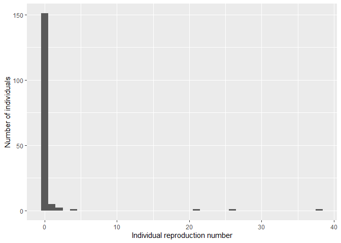
We can see from visual inspection that this distribution is highly over-dispersed (high “superspreading”).
To fit a negative binomial distribution to this data and estimate the dispersion parameter (which indicates the degree of superspreading), we use the fitdistrplus package. We then calculate the 95% confidence intervals using the standard error estimates and the lower and upper quantiles of the Normal distribution that correspond to a 95% interval.
library(fitdistrplus)

## fit distribution
fit <- fitdist(r_i, "nbinom")

## extract the "size" parameter
mid <- fit$estimate[["size"]]

## calculate the 95% confidence intervals using the standard error estimate and
## the 0.025 and 0.975 quantiles of the normal distribution.
lower <- mid + fit$sd[["size"]]*qnorm(0.025)
upper <- mid + fit$sd[["size"]]*qnorm(0.975)

round(mid, 4)
#> [1] 0.0204
round(lower, 4)
#> [1] 0.0061
round(upper, 4)
#> [1] 0.0347
We can see that the dispersion parameter is estimated as 0.020 (95% CI 0.006 - 0.035). As this value is significantly lower than one, we can conclude that the degree of super-spreading is high. This is in line with visual inspection of the histogram made above.
2 Likes